AM–FM Models
A component set Array{Tuple{Function,Function,Real},1} maps to an AM–FM model AMFMmodel.
This mapping is provided in the ISA module.
using ISADefining an AM–FM Model
We can define an AM–FM model as follows. First, define a component set.
a₀(t) = exp(-t^2)
ω₀(t) = 2.0
φ₀ = 0.0
𝐶₀ = (a₀,ω₀,φ₀)

a₁(t) = 1.0
ω₁(t) = 10*t
φ₁ = 0.1
𝐶₁ = (a₁,ω₁,φ₁)

a₂(t) = 0.8*cos(2t)
ω₂(t) = 10 + 7.5*sin(t)
φ₂ = π
𝐶₂ = (a₂,ω₂,φ₂)

𝑆 = [𝐶₀,𝐶₁,𝐶₂]
Then, pass the component set to the function AMFMmodel().
z = AMFMmodel(𝑆)We also allow an AM–FM model AMFMmodel to be defined by passing an array of AMFMcomp to the function AMFMmodel(). First, define the components.
a₀(t) = exp(-t^2)
ω₀(t) = 2.0
φ₀ = 0.0
ψ₀ = AMFMcomp(a₀,ω₀,φ₀)

a₁(t) = 1.0
ω₁(t) = 10*t
φ₁ = 0.1
ψ₁ = AMFMcomp(a₁,ω₁,φ₁)

a₂(t) = 0.8*cos(2t)
ω₂(t) = 10 + 7.5*sin(t)
φ₂ = π
ψ₂ = AMFMcomp(a₂,ω₂,φ₂)
Then pass the array of AMFMcomp to the function AMFMmodel().
z = AMFMmodel([ψ₀,ψ₁,ψ₂])Evaluating an AM–FM Model
Once an AM–FM model AMFMmodel is defined it can be evaluated at a time instant Float64
julia> t₀ = 0.15
julia> z(t₀)
-0.1844131722041218 + 1.146808452231523im
or over a range of time instants Array{Float64,1}.
julia> t = 0.0:0.25:1.0
julia> z(t)
5-element Array{Complex{Float64},1}:
  2.3127623746121317 + 1.2092678279852234im
 -1.2963995650827416 + 0.025282127799684584im
  0.5931797251405191 + 0.9674372363846413im
 0.25073410019471093 - 0.5690871746595758im
  1.4587415832942454 + 0.7649782375222325im
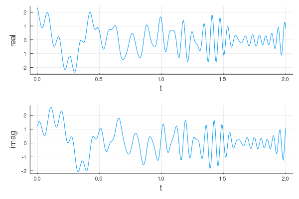
Another example of evaluating an AM–FM model over a range of time instants using the Plots module follows.
using Plots
t = 0.0:0.005:2.0
p1 = plot(t, real(z(t)), xlab="t", ylab="real", legend = :false)
p2 = plot(t, imag(z(t)), xlab="t", ylab="imag", legend = :false)
plot(p1, p2, layout = (2,1))